Cassandra Basics
Flow Diagram
A flow diagram that overviews the setup for a Cassandra simulation is displayed
in Fig. 1. This diagram employs two automation scripts located
in the /Scripts/ directory: mcfgen.py and library_setup.py. These
scripts are particularly useful when simulating large molecules. For details
about how to use them, please refer to sections sec:mcfgen and sec:libgen of
this user guide, and to the README files located in the subdirectories inside
the directory /Scripts/.
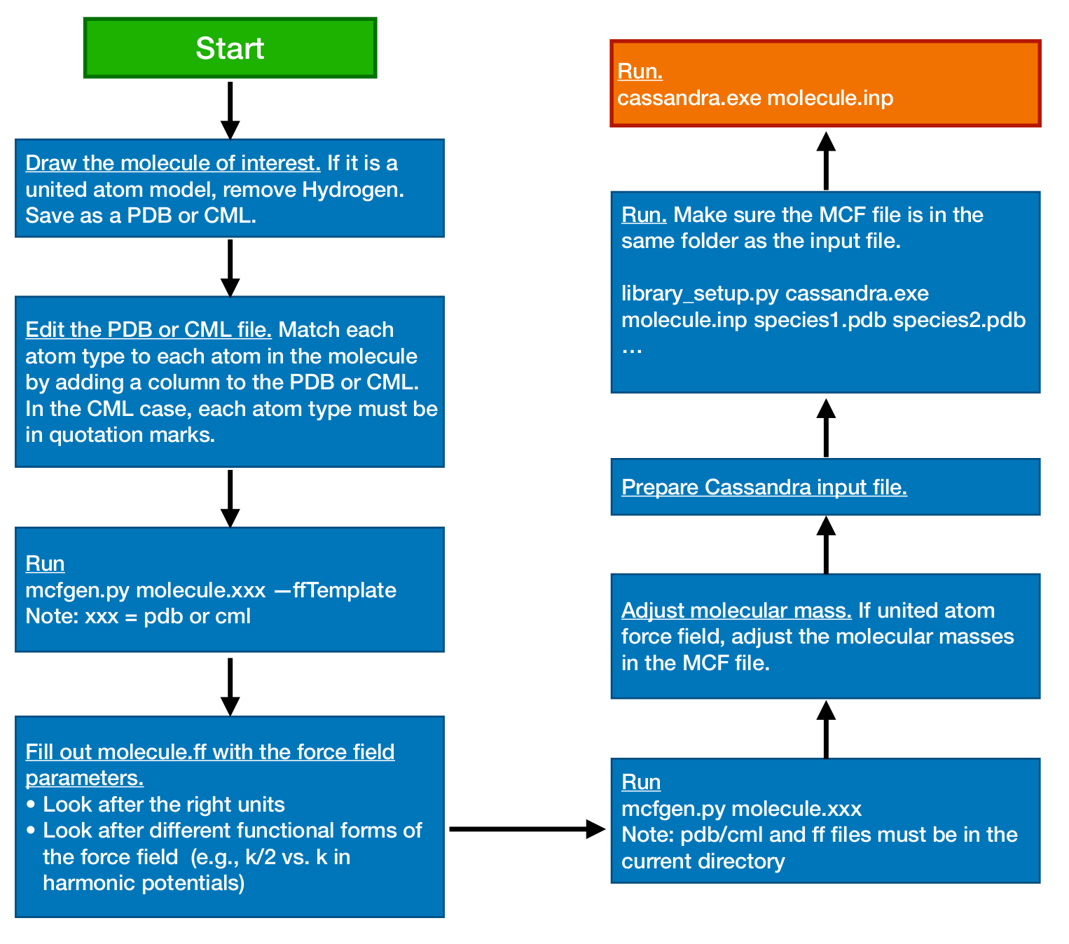
Fig. 1 Flow diagram representing a typical setup of a Cassandra simulation
Cassandra Simulation Setup
Once a system is identified, setting up a Cassandra simulation from scratch requires preparation of the following files.
- A molecular connectivity file (MCF) (
*.mcf) containing the molecular connectivity information on bonds, angles, dihedrals, impropers and whether the molecule is composed of fragments. For information on the MCF file, please refer to Molecular Connectivity File. - An input file (
*.inp) (see Simulation Input File) - If the molecule is composed of fragments, then a fragment library file for each of the fragments is required. For instructions on how to generate these files, please refer to Generate Library of Fragment Configurations.
MCF files for united-atom models of methane, isobutane, dimethylhexane,
cyclohexane and diethylether are provided in the MCF directory. Input
files for NVT, NPT, GCMC and GEMC ensembles are located in the Examples
directory which also contains fragment library files for a number of molecules
simulated in these ensembles.
Cassandra File Preparation
MCF File
One MCF file is required for each unique species in a simulation. A species is
defined as a collection of atoms associated with each other through bonds. Thus
a molecule is a species as is an ion. If you wanted to simulate sodium sulfate,
you would need separate MCF files for the sodium ion and the sulfate ion. MCF
files can be created manually or by using the scripts provided with the code, as
described in the section Generate a Molecular Connectivity File. Instructions for generating an MCF
file can also be found in the Scripts/MCF_Generation/README file.
Input File
An input file is required for a Cassandra simulation. The input file specifies conditions for the simulation and various keywords required for the simulation in a given ensemble. Please refer to Simulation Input File for further details.
Fragment Library Generation
Cassandra makes use of reservoir sampling schemes to correctly and efficiently sample the various coupled intramolecular degrees of freedom associated with branch points and rings. For more information, please see Ref. cite{Shah:2011}. The molecule is decomposed into fragments that are either branch points or ring groups, each coupled to other fragments via a single dihedral angle. Thus, the total number of fragments of a molecule is the sum of branch points and ring groups in the molecule. The neighboring fragments are connected by two common atoms present in each of the fragments. Note that the ring group contains all the ring atoms and those directly bonded to the ring atoms. For each fragment identified, Cassandra runs a pre-simulation in the gas phase to sample the intramolecular degrees of freedom. A library of a large number of these conformations are stored for use in an actual simulation.
The gas phase library generation has been automated with the script
library_setup.py located in the Scripts/Frag_Library_Setup
directory. Use the following command for generating the fragment library:
python $PATH/Frag_Library_Setup/library_setup.py $PATH/Src/cassandra_executable input_filename mol1.pdb (mol1.cml) mol2.pdb (mol2.cml) ...}
where input_filename is the name of the input file for the actual simulation
and mol1.pdb mol2.pdb ... or mol1.cml mol2.cml ...} correspond to the
names of the pdb (or cml) files used to generated the MCF files. Make sure that
if a file does not exist in the current working directory, its path relative to
the current working directory is specified.
Running a Simulation
To launch a Cassandra simulation, run the following command:
cassandra_executable input_filename
The executable will read input_filename and execute the instructions. Make
sure that the required files (MCF, fragment library files) are located in the
directories as given in the input file.
Restarting a Simulation
Restarting a simulation requires either a checkpoint file (*.chk produced by
Cassandra) or a configuration file obtained from xyz files generated from a
previous simulation. Please refer to Start Type to find
information about the keywords checkpoint and read_config.
Cassandra Output Files
Cassandra generates several output files which can be used for later analysis.
All have as a prefix the Run_Name specified in the input file.
See Run Name for details. The type of output is specified by the
file name suffix. The following are generated:
- Log file (
*.log): Contains basic information on what the run is, timing information and reports the various parameters specified by the user. A complete copy of the input file is reproduced. Other important information includes the move acceptance rates. You can use the log file to keep track of what conditions were simulated. - Coordinate file (
*.xyzor*.box#.xyz): For each box in the system, a set of xyz coordinates are written out with a frequency specified by the user (Coord_Freq). The file has as a header the number of atoms in the box. Following this, the atomic coordinates of molecule 1 of species 1 are written, then the coordinates of molecule 2 of species 1 are written, etc. After all the coordinates of the molecules of species 1 are written, the coordinates of the molecules of species 2 are written, etc. You can use this file to do all your structural analysis and post processing.
Note
Note that if you generate your initial configuration using the make_config
command, the first ‘’snapshot’’ of the coordinate file will contain the initial
configuration of all the species in the system for a given box. You can use this
configuration to check on whether the initial configuration is reasonable, or
use it as an input to other codes. Note that the initial configuration will be
generated using a configurational biased scheme, so it may be a better starting
configuration than if you used other methods.
- Checkpoint file (
*.chk): A checkpoint file is written everyCoord_Freqsteps. This can be used to restart a simulation from this point using all of the same information as the run that was used to generate the checkpoint file. To do this, you must use the checkpoint restart option (see Start Type. It will basically pick up where the simulation left off, using the same random number seed, maximum displacements, etc. This is useful in case your job crashes and you want to continue running a job. You can also use the checkpoint file to start a new simulation using the configuration of the checkpoint file as an initial configuration and the optimized maximum displacements. To do this, use the scriptread_old.py. You will need to set a new random number seed if you do this. See the documentation in Starting Seed for more details. - H-matrix file (
*.Hor*.box#.H): This file is written to everyCoord_FreqMC steps. The first line is the box volume in angstrom3. The next three lines are the box coordinates in angstrom in an H-matrix form. Since Cassandra only supports cubic boxes at the moment, this is just a diagonal and symmetric matrix, but is included here for later versions that will enable non-orthogonal boxes. After this, a blank line is written. The next line is the box number, and the final line(s) is(are) the species ID and number of molecules for that species in this box. If there are three species, there will be three lines. This output is repeated everyCoord_Freqtimes. This file allows you to compute the density of the box during constant pressure simulations. - Property file (
*.prp#or*.box#.prp#): This file lists the instantaneous thermodynamic and state properties for each box. Note that you can have more than one property file (hence the # after ‘prp’) and more than one box (also why there is a # after ‘box’). The user specifies which properties are to be written and in what order, and these are then reproduced in this file. The file is written to everyProp_Freqsteps. A header is written to the first two lines to designate what each property is. You may use this file to compute thermodynamic averages. - Widom property file (
*.spec#.wprpor*.spec#.box#.wprp): This file lists the averagewidom_var(defined in CBMC Widom Insertion Method) for each system configuration (step) in which Widom insertions are performed for a given species and a given box. The species number is the#in.spec#in the file extension. For a multi-box system, the box number is the#in.box#. The first column contains the number of MC steps or sweeps that have been completed when the Widom insertions are performed and the second column contains the averagewidom_varfor that step. - Secondary Widom property file (
*.spec#.wprp2*.spec#.box#.wprp2): This file lists the averagewidom_var(defined in CBMC Widom Insertion Method) for each Widom insertion subgroup in each system configuration (step) in which Widom insertions are performed for a given species and a given box. The naming convention is analogous to that of normal Widom property files. There is one row (line) per system configuration (frame) in which Widom insertions are performed for the species and box, and one column per subgroup per Widom insertion frame. Unlike basic Widom property files, these do not have row or column labels, and do not include the step number or sweep number, but the step number or sweep number corresponding to each row is the same as in the Widom property file. Further details are given in Widom Insertion).